Exploring Excel's Hidden Treasures: LET and LAMBDA Functions
January 31, 2023
by David H. Ringstrom, CPA

Many Excel formulas are quite manageable, but sometimes a formula can end up spanning two or more rows in Excel's formula bar. Such formulas are tricky to audit and to edit because they often repeat calculations in two or more places.
In this article you'll see how the LET function will enable you to document formulas and eliminate repetitive calculations in Excel 2021 and Microsoft 365. What's more, you may have complex formulas that are hard to reuse in other spreadsheets because of their complexity. I'll show you how the LAMBDA function in Microsoft 365 enables you to create custom reusable worksheet functions. Before we get to LET and LAMBDA let's first review how to name worksheet cells, which works in all versions of Excel, as groundwork. As you'll see we'll calculate the volume of a box several different ways so that you can compare and contrast the techniques.
BUILDING THE SPREADSHEET
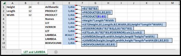
Enter the data shown in cells A1:E4 of Figure 1 into a blank spreadsheet, or download the spreadsheet by clicking on the chart below.
The PRODUCT function multiplies either individual values or ranges of values together in the same fashion as carrying out direct multiplication. This serves as foreshadowing for how LAMBDA functions work, as you will be able to pass information in a similar fashion to your custom worksheet functions. Next enter the formula =FORMULATEXT(E1) in cell F1 and then copy the formula down to cell F3 to display the formulas in cells E1:E3. FORMULATEXT returns #N/A if the cell you reference does not contain a formula, and returns #NAME? in Excel 2010 and earlier.
Most Excel formulas utilize cell addresses in this fashion, as most Excel users are not aware of the concept of naming cells. You can use names interchangeably with cell references, the difference being that names within formulas make it easier to comprehend formulas. The LET function uses a similar concept, although the names only exist within the context of that specific formula. LAMBDA functions utilize parameters, which again serve a similar function.
Click here to download a working spreadsheet.
NAMING WORKSHEET CELLS
Let's compare three different approaches for assigning names to cells:
- Select cell B1 and then choose Formulas | Define Name. The Define Name dialog box surmises that you want to assign the text in A1 as a name for cell B1, which you can override if needed, and then click OK.
- Select cell B2 and then click into the Name Box, which appears just above the top left-hand corner of the worksheet frame. Type the word Width into the field and press Enter.
- Select cells A3:B3, choose Formulas | Create from Selection. Left Column will be preselected, when means when you click OK Excel will assign the text in the left column of the cell the right column. Click OK to confirm this action.
We could have used Create from Selection to assign all three names at once, but we'll be using the Define Name command to create LAMBDA functions. Names that you assign to cells will appear in the Name Box when you click on a given cell. Further, you can navigate to a specific name anywhere in a workbook by clicking the arrow in the Name Box and then selecting any name from the list.
Next enter the following text and formula:
Cell D4: Names
Cell E4: =Length*Width*Height
You can enter this formula in a couple of different ways:
- Type an equal sign and then navigate to each cell. Excel will display the name instead of the cell reference as you write the formula.
- Press F3 in Excel for Windows to display the Paste Names dialog box or choose Formulas | Use in Formula (unfortunately neither of these options are available in Excel for Mac).
- Type an equal sign and then start typing the first part of a name you have assigned. You can select the name from the AutoComplete list, type out the name in full, or press the Tab key to finish out the name once you've entered enough characters to create a match.
Names can be comprised of as little as a single letter. Names must begin with a letter or underscore, cannot contain spaces, and can contain numbers if the name does not correspond to a cell reference. For instance, TAX2023 is not a valid name but TAX_2023 is.
Copy the formula in cell F3 down to cell F4 so that you can compare the approaches. As you can see, names enable you to determine what a formula refers to with a glance, as opposed to chasing down each cell reference. Further names within formulas are absolute references, meaning if you copy the formula down or across the formula will always refer to the named cell(s), unlike cell references where the row number and or column letter changes unless prefaced by an $ to create an absolute or mixed reference.
INTRODUCING THE LET FUNCTION
The LET function enables you to establish up to 126 variables, along with one calculation. The calculation needn't reference all the variables, although typically it will. Variables are established in name pairs, where you assign a name and then a value. Variable names exist only in the context of the individual formula, so as you’ll see we can use Length, Width, and Height within our LET in a different context from the names that we assigned earlier. Enter the following information:
Cell D5: LET
Cell E5: =LET(Height,B1,Length,B2,Width,B3,Height*Length *Width)
The formula breaks down as follows:
- Name1: Height is our first variable name we're assigning to Height
- Name_value1: Cell B1 contains the value that we’re assigning to Height
- Name2: Length is our second variable name
- Name_value2: Cell B2 contains the value that we're assigning to Length
- Name3: Width is our third variable name
- Name_value3: Cell B3 contains the value that we're assigning to Width
- Calculation_or Name4: Enter a calculation after you have established the Name and Name_value pairs.
The rules for names within the LET function are like assigning names to worksheet cells: names cannot correspond to a cell reference, must begin either a letter or underscore, and cannot contain spaces. These names will not appear in the Name Box or the Name Manager. The LET function will return #NAME? if your calculation includes a name that you did not assign within the formula or that you misspelled.
Although LET is useful for documenting formulas, an even better use eliminates repetitive calculations within formulas. Enter the following into the respective cells:
Cell D6: ISERROR
Cell E6: =IF(ISERROR(B1*B2*B3),0,B1*B2*B3)
The IF function has the following three arguments:
- Logical_test: a calculation that returns TRUE or FALSE. In this case ISERROR is determining if B1*B2*B3 results in an error such as #VALUE! when a user enters text or a space into cells B1, B2, or B3.
- Value_if_true: In this case if ISERROR returns TRUE we want to return a zero.
- Value_if_false: If ISERROR returns FALSE then we want to carry out the calculation B1*B2*B3.
This simple example illustrates how often we end up repeating the same calculation one or more times within a formula. This can make formulas harder to comprehend and harder to edit as well, which raises the specter of spreadsheet errors if edits are not carried out consistently through the formula. This brings us to how LET eliminates repetitive calculations. Enter this formula into cell E7: =LET(calc,B1*B2*B3,IF(ISERROR(calc),0 ,calc)). Now let’s break the formula down:
- Name1: calc is the generic name that I use for calculations such as this.
- Name_value1: B1*B2*B3 shows that name values within LET can be inputs or calculations
- Calculation_or_Name2: IF(ISERROR(calc),0,calc) shows that we can use the word calc as a placeholder for B1*B2*B3. This means that if we need to edit the formula later, we only must edit the Name_value1 argument instead of making multiple edits.
Keep in mind that I used the IF/ISERROR combination as a vehicle to explain LET. The IFERROR function is a better alternative for managing many common errors. Enter this formula in cell F8: =IFERROR(B1*B2*B3,0). IFERROR has two arguments: value, which represents a calculation, and value_if_error, which represents an alternate value, text, or calculation to use if the value argument returns an error.
INTRODUCING THE LAMBDA FUNCTION
The downside of LET is that you must write each formula from scratch repeatedly. Conversely, the LAMBDA function enables you to formalize the formula so that you simply pass information to a custom worksheet function instead of constantly reinventing the wheel. There are four stages to writing a LAMDBA formula:
- Writing the formula in a worksheet cell.
- Passing test values to the formula in the worksheet cell.
- Formalizing the LAMBDA by using the Define Name command.
- Utilizing your custom worksheet function in your worksheet.
Enter the following, which I’ll warn you in advance will result in a #CALC! error in cell E8 if you’ve entered everything properly:
Cell D8: LAMBDA
Cell E8: =LAMBDA(length,width,height,length*height*width)
Let's break down the formula first, and then I'll explain why it returns #CALC!:
- Parameter_or_calculation: Our first parameter is height.
- Parameter_or_calculation: Our second parameter is width.
- Parameter_or_calculation: Our third parameter is length.
- Parameter_or_calculation: Our calculation is height*width*length.
The reason that the formula returns #CALC! is that we haven't provided any values for it to reference, which we'll do on the next row:
Cell D9: LAMBDA
Cell E9: =LAMBDA (height,length,width,height*length*width) (B1,B2,B3)
Notice that you can copy the formula from row 9 down to row 10 and then add the test values (B1,B2,B3) to the end of the formula, which when you press Enter should return 3,456. Once you have tested your LAMBDA, you can now formalize it:
- Click on cell E8 and then copy the entire formula within the formula bar, including the equal sign. If you use cell E9, copy everything except the test values at the end, meaning (B1,B2,B3).
- Choose Formulas | Define Name.
- Enter a name such as BOXVOLUME in the Name field.
- Enter "Computes the volume of a box" in the Comment field.
- Paste the formula you copied in step 1 into the Refers To field.
- Click OK.
Now enter the following:
Cell D10: BOXVOLUME
CELL E10: =BOXVOLUME(B1,B2,B3)
You can now use the BOXVOLUME function anywhere in this workbook. You can transfer the function to other workbooks by copying one or more cells that contain named LAMBDA functions, such as BOXVOLUME, or copying or moving a worksheet that contains such formulas. Remember, LAMBDA functions only work in Microsoft 365 and will return #NAME? in earlier versions of Excel. I've only had space to show you to the tip of the iceberg here regarding what's possible with LAMBDA, but hopefully you can imagine the possibilities.
INTRODUCING THE NAME MANAGER
Now let's choose Formulas | Name Manager. This dialog box enables you to manage names that you've assigned in your workbooks and will enable you to manage LAMBDA functions you create as well. The Name Manager enables you to add, delete, or edit new names and LAMBDA functions. One downside of using names in formulas is that deleted names cause formulas to return #NAME?. To see this in action:
- Click the Delete button within the Name Manager to delete the Height name.
- Click OK to confirm the deletion and then click Close.
- The formula in cell E4 will now return #NAME? instead of 3,456. Notice that the formula in cell E5 is not affected because LET maintains its own context for names.
To repair the formula in cell E5 you may either update the formula to use a cell reference or create the name again. Doing so will cause the formula to return 3,456 again.
I hope that I have helped you expand your Excel toolbox. Some years ago I coined the phrase "Either you work Excel, or it works you!" Utilizing features such as naming cells, and functions such as LET and LAMBDA are surefire ways to turn the tide and ensure that you're not getting pushed around by Excel and are working more effectively.

David Ringstrom (www.davidringstrom.com) is the author of Exploring Microsoft Excel’s Hidden Treasures: Turbocharge your Excel proficiency with expert tips, automation techniques, and overlooked features. David has worked as a spreadsheet consultant for over 30 years and has taught over 2,000 live webinars.
This article appears in the winter 2023 issue of the Washington CPA magazine. Read more here.